Intro to the OpenOA `PlantData` and QA Methods#

In this example we will be using the ENGIE open data set for the La Haute Borne wind power plant, and demonstrating how to use the quality assurance (QA) methods in OpenOA to help get this data ready for use with the PlantData class. This notebook will walk through the creation of the project_Engie module, especially the prepare() method that returns either the cleaned data or a PlantData object.

While we work with project_ENGIE.py to standardize the QCing of the La Haute Borne data, it should be noted that the use of an external script to load in data is entirely optional. For instance, a user could do all their work in a single script, set up a template Jupyter Notebook for working with data, or any other means that produces the data that can be read into PlantData and the associated metadata (PlantMetaData), as determined by the user input data.

The `PlantData` object#

The PlantData object is the core data structure for OpenOA, which is used for importing and validating wind power plant operational data for analysis in OpenOA.

What’s changed in v3?#

For users that are well acquainted with OpenOA and its data structures, there are a few changes to the ways the code now operates:

All data objects such as PlantData.scada are pandas DataFrames now, so there is no longer the need to access the data via PlantData.scada._df
Because all data objects are pandas DataFrames, AssetData and ReanalysisData have been dropped in favor of: PlantData.asset and PlantData.reanalysis, respectively.
Reanalysis data is the only data object that diverges, and is now a dictionary of DataFrames, which enables the use of an arbitrary number of reanalysis products to be imported and used
There are now a number of convenience methods, such as PlantData.turbine_ids, PlantData.tower_ids, PlantData.turbine_df(), and PlantData.tower_df() for commonly used data access routines.
PlantData is now accompanied by a PlantMetaData object that is powered by dictionaries to help routinely set up mappings between user data formats and OpenOA internal formats that use an IEC-25 schematic.

`PlantData` and `PlantMetaData` 101#

The PlantData object, as previously stated, is the central data repository and object for working with operational data in OpenOA. All of the analysis methods are built around this object for both API consistency and to make OpenOA easily extensible to new/more analysis methods. For the OpenOA examples, the metadatafile: data/plant_meta.yml will be used (and a JSON reference for those that prefer JSON: data/plant_meta.json) to map the La Haute Borne fields to the OpenOA fields. This v3 update allows a user to bring their data directly into a PlantData object with a means for the OpenOA to know which data fields are being used

Below is a demonstration of loading a PlantMetaDataobject directly to show what data are expected, though there is a PlantMetaData.load() that can accept a dictionary or file path input for routinized workflows.

metadata = PlantMetaData(
    latitude,  # float
    longitude,  # float
    scada,  # dictionary of column mappings and data frequency
    meter,  # dictionary of column mappings and data frequency
    tower,  # dictionary of column mappings and data frequency
    status,  # dictionary of column mappings and data frequency
    curtail,  # dictionary of column mappings and data frequency
    asset,  # dictionary of column mappings
    reanalysis,  # dictionary of each product's dictionary of column mappings and data frequency
)

For each of the data objects above, there is a corresponding meta data class to help guide users. For instance, the SCADAMetaData (below) has pre-set attributes to help guide users outside of the docstrings and standard documentation. The other meta data objects are: MeterMetaData, TowerMetaData, StatusMetaData, CurtailMetaData, AssetMetaData, and ReanalysisMetaData (one is created for each producted provided).

For example, each of the metadata classes allows inputs for the column mappings and timestamp frequency to enable the data validation steps outlined in the process summary. However to clarify the units and data types expected, each of the metadata classes contains the immutable attributes: units and dtypes, as shown below for the SCADAMetaData class, to signal to users what units each data input should be in, when passed, and what type the data should be able to be converted to, if it’s not already in that format. Some examples of acceptable formats would be string-encode floats, or string-encoded timestamps, both of which can be automatically converted in the initialization steps.

from pprint import pprint
from openoa.schema import SCADAMetaData

scada_meta = SCADAMetaData()  # no inputs means use the default, internal mappings
print("Expected units for each column in the SCADA data:")
pprint(scada_meta.units)
print()
print("Expected data types for each column in the SCADA data:")
pprint(scada_meta.dtypes)

Expected units for each column in the SCADA data:
{'WMET_EnvTmp': 'C',
 'WMET_HorWdDir': 'deg',
 'WMET_HorWdDirRel': 'deg',
 'WMET_HorWdSpd': 'm/s',
 'WROT_BlPthAngVal': 'deg',
 'WTUR_SupWh': 'kWh',
 'WTUR_TurSt': None,
 'WTUR_W': 'kW',
 'asset_id': None,
 'time': 'datetim64[ns]'}

Expected data types for each column in the SCADA data:
{'WMET_EnvTmp': <class 'float'>,
 'WMET_HorWdDir': <class 'float'>,
 'WMET_HorWdDirRel': <class 'float'>,
 'WMET_HorWdSpd': <class 'float'>,
 'WROT_BlPthAngVal': <class 'float'>,
 'WTUR_SupWh': <class 'float'>,
 'WTUR_TurSt': <class 'str'>,
 'WTUR_W': <class 'float'>,
 'asset_id': <class 'str'>,
 'time': <class 'numpy.datetime64'>}

Below is a demonstration of loading a PlantData object directly, though there are class methods for loading from file or an ENTR warehouse.

plant = PlantData(
    metadata,  # PlantMetaData, dictionary, or file
    analysis_type,  # list of analysis types expected to be performed, "all", or None
    scada,  # None, DataFrame or CSV file path
    meter,  # None, DataFrame or CSV file path
    tower,  # None, DataFrame or CSV file path
    status,  # None, DataFrame or CSV file path
    curtail,  # None, DataFrame or CSV file path
    asset,  # None, DataFrame or CSV file path
    reanalysis,  # None, dictionary of DataFrames or CSV file paths with the name of the product for keys
)

On loading, the data will be validated automatically according to the analysis_type input(s) provided to ensure columns exist with the expected names, data types are correct, and data frequencies are of a sufficient resolution. However, while all erros in this process are caught, only those of concern to an analysis_type are raised, with the exception of “all” raises any error found and None ignore all errors.

Imports#

from pprint import pprint

import numpy as np
import pandas as pd
from matplotlib import pyplot as plt

from openoa import PlantData
from openoa.utils import qa
from openoa.utils import plot

import project_ENGIE

# Avoid clipping data previews unnecessarily
pd.set_option("display.max_rows", 100)
pd.set_option("display.max_columns", 100)

WARNING:py.warnings:/Users/rhammond/miniforge3/envs/openoa/lib/python3.11/site-packages/h5pyd/version.py:23: DeprecationWarning: distutils Version classes are deprecated. Use packaging.version instead.
  _exp = _sv(version)

QA’ing ENGIE’s open data set#

ENGIE provides access to the data of its ‘La Haute Borne’ wind farm through https://opendata-renewables.engie.com and through an API. The data gives users the opportunity to work with real-world operational data.

The series of notebooks in the ‘examples’ folder uses SCADA data downloaded from https://opendata-renewables.engie.com, saved in the examples/data folder. Additional plant level meter, availability, and curtailment data were synthesized based on the SCADA data.

The data used throughout these examples are pre-processed appropriately for the issues described in the subsequent sections, and synthesized into a routinized format in the examples/project_ENGIE.py Python script.

Note: This demonstration is centered around a specific data set, so it should be noted that there are other methods for working with data that are not featured here, and we would like to point the user to the API documentation for further data checking and manipulation methods.

Step 1: Load the SCADA data#

First we’ll need to unzip the data, and read the SCADA data to a pandas DataFrame so we can take a look at the data before we can start working with it. Here the project_ENGIE.extract_data() method is used to unzip the data folder because this demonstration is based on working with the ENGIE provided data without any preprocessing steps taken.

data_path = "data/la_haute_borne"
project_ENGIE.extract_data(data_path)

scada_df = pd.read_csv(f"{data_path}/la-haute-borne-data-2014-2015.csv")

scada_df.head(10)

	Wind_turbine_name	Date_time	Ba_avg	P_avg	Ws_avg	Va_avg	Ot_avg	Ya_avg	Wa_avg
0	R80736	2014-01-01T01:00:00+01:00	-1.00	642.78003	7.12	0.66	4.69	181.34000	182.00999
1	R80721	2014-01-01T01:00:00+01:00	-1.01	441.06000	6.39	-2.48	4.94	179.82001	177.36000
2	R80790	2014-01-01T01:00:00+01:00	-0.96	658.53003	7.11	1.07	4.55	172.39000	173.50999
3	R80711	2014-01-01T01:00:00+01:00	-0.93	514.23999	6.87	6.95	4.30	172.77000	179.72000
4	R80790	2014-01-01T01:10:00+01:00	-0.96	640.23999	7.01	-1.90	4.68	172.39000	170.46001
5	R80736	2014-01-01T01:10:00+01:00	-1.00	511.59000	6.69	-3.34	4.70	181.34000	178.02000
6	R80711	2014-01-01T01:10:00+01:00	-0.93	692.33002	7.68	4.72	4.38	172.77000	177.49001
7	R80721	2014-01-01T01:10:00+01:00	-1.01	457.76001	6.48	-4.93	5.02	179.82001	174.91000
8	R80711	2014-01-01T01:20:00+01:00	-0.93	580.12000	7.35	6.84	4.20	172.77000	179.59000
9	R80721	2014-01-01T01:20:00+01:00	-1.01	396.26001	6.16	-1.94	4.88	179.82001	177.85001

The timestamps in the column Date_time show that we have timezone information encoded, and that the data have a 10 minute frequency to them (or “10min” according to the pandas guidance: https://pandas.pydata.org/pandas-docs/stable/user_guide/timeseries.html#timeseries-offset-aliases)

To demonstrate the breadth of data that the QA methods are inteneded to handle this demonstration will step through the data using the current format, and an alternative where the timezone data has been stripped out.

scada_df_tz = scada_df.loc[:, :].copy()  # timezone aware
scada_df_no_tz = scada_df.loc[:, :].copy()  # timezone unaware

# Remove the timezone information from the timezone unaware example dataframe
scada_df_no_tz.Date_time = scada_df_no_tz.Date_time.str[:19].str.replace("T", " ")

# # Show the resulting change
scada_df_no_tz.head()

	Wind_turbine_name	Date_time	Ba_avg	P_avg	Ws_avg	Va_avg	Ot_avg	Ya_avg	Wa_avg
0	R80736	2014-01-01 01:00:00	-1.00	642.78003	7.12	0.66	4.69	181.34000	182.00999
1	R80721	2014-01-01 01:00:00	-1.01	441.06000	6.39	-2.48	4.94	179.82001	177.36000
2	R80790	2014-01-01 01:00:00	-0.96	658.53003	7.11	1.07	4.55	172.39000	173.50999
3	R80711	2014-01-01 01:00:00	-0.93	514.23999	6.87	6.95	4.30	172.77000	179.72000
4	R80790	2014-01-01 01:10:00	-0.96	640.23999	7.01	-1.90	4.68	172.39000	170.46001

Below, we can see the data types for each of the columns. We should note that the timestamps are not correctly encoded, but are considered as objects at this time

scada_df_tz.dtypes

Wind_turbine_name     object
Date_time             object
Ba_avg               float64
P_avg                float64
Ws_avg               float64
Va_avg               float64
Ot_avg               float64
Ya_avg               float64
Wa_avg               float64
dtype: object

scada_df_no_tz.dtypes

Wind_turbine_name     object
Date_time             object
Ba_avg               float64
P_avg                float64
Ws_avg               float64
Va_avg               float64
Ot_avg               float64
Ya_avg               float64
Wa_avg               float64
dtype: object

Step 2: Convert the timestamps to proper timestamp data objects#

Using the qa.convert_datetime_column() method, we can convert the timestamp data accordingly and insert the UTC-encoded data as an index for both the timezone aware, and timezone unaware data sets.

Under the hood this method does a few helpful items to create the resulting data set:

Converts the column “Date_time” to a datetime object
Creates the new datetime columns: “Date_time_localized” and “Date_time_utc” for the localized and UTC-encoded datetime objects
Sets the UTC timestamp as the index
Creates the column “utc_offset” containing the difference between the UTC timestamp and the localized timestamp that will be used to determine if the timestamp is in DST or not.
Creates the column “is_dst” indicating if the timestamps are in DST (True), or not (False) that will be used later when trying to assess time gaps and duplications in the data

Notice that in the resulting data that the data type of the column “Date_time” is successfully made into a localized timestamp in the timezone aware example, but is kept as a non-localized timestamp in the unaware example.

In the below, the “Date_time_utc” column should always remain in UTC time and the “Date_time_localized” column should always remain in the localized time. Conveniently, Pandas provides two methods tz_convert() and tz_localize() to toggle back and forth between timezones, which will operate on the index of the DataFrame. It is worth noting that the local time could also be UTC, in which case the two columns would be redundant.

The localized time, even when the passed data is unaware, is adjusted using the local_tz keyword argument to help normalize the time strings, from which a UTC-based timestamp is created (even when local is also UTC). By calculating the UTC time from the local time, we are able to ascertain DST shifts in the data, and better assess any anomalies that may exist.

However, there may be cases where the timezone is neither encoded (the unaware example), nor known. In the former, we can use the local_tz keyword argument that is seen in the code above, but for the latter, this is much more difficult, and the default value of UTC may not be accurate. In this latter case it is useful to try multiple timezones, such as an operating/owner company’s headquarters or often the windfarm’s location to find a best fit.

Note: In the case of US-based wind power plants, the "qa.wtk_xx()" methods, such as "qa.wtk_diurnal_prep()" and "qa.wtk_diurnal_plot()", can be used for working with NREL's WINDToolKit for further data checking, validation, and plotting.

scada_df_tz = qa.convert_datetime_column(
    df=scada_df_tz,
    time_col="Date_time",
    local_tz="Europe/Paris",
    tz_aware=True # Indicate that we can use encoded data to convert between timezones
)
scada_df_tz.head()

	Wind_turbine_name	Date_time	Ba_avg	P_avg	Ws_avg	Va_avg	Ot_avg	Ya_avg	Wa_avg	Date_time_localized	Date_time_utc	utc_offset	is_dst
Date_time_utc
2014-01-01 00:00:00+00:00	R80736	2014-01-01 01:00:00+01:00	-1.00	642.78003	7.12	0.66	4.69	181.34000	182.00999	2014-01-01 01:00:00+01:00	2014-01-01 00:00:00+00:00	0 days 01:00:00	False
2014-01-01 00:00:00+00:00	R80721	2014-01-01 01:00:00+01:00	-1.01	441.06000	6.39	-2.48	4.94	179.82001	177.36000	2014-01-01 01:00:00+01:00	2014-01-01 00:00:00+00:00	0 days 01:00:00	False
2014-01-01 00:00:00+00:00	R80790	2014-01-01 01:00:00+01:00	-0.96	658.53003	7.11	1.07	4.55	172.39000	173.50999	2014-01-01 01:00:00+01:00	2014-01-01 00:00:00+00:00	0 days 01:00:00	False
2014-01-01 00:00:00+00:00	R80711	2014-01-01 01:00:00+01:00	-0.93	514.23999	6.87	6.95	4.30	172.77000	179.72000	2014-01-01 01:00:00+01:00	2014-01-01 00:00:00+00:00	0 days 01:00:00	False
2014-01-01 00:10:00+00:00	R80790	2014-01-01 01:10:00+01:00	-0.96	640.23999	7.01	-1.90	4.68	172.39000	170.46001	2014-01-01 01:10:00+01:00	2014-01-01 00:10:00+00:00	0 days 01:00:00	False

print(scada_df_tz.index.dtype)
scada_df_tz.dtypes

datetime64[ns, UTC]

Wind_turbine_name                            object
Date_time              datetime64[ns, Europe/Paris]
Ba_avg                                      float64
P_avg                                       float64
Ws_avg                                      float64
Va_avg                                      float64
Ot_avg                                      float64
Ya_avg                                      float64
Wa_avg                                      float64
Date_time_localized    datetime64[ns, Europe/Paris]
Date_time_utc                   datetime64[ns, UTC]
utc_offset                          timedelta64[ns]
is_dst                                         bool
dtype: object

scada_df_no_tz = qa.convert_datetime_column(
    df=scada_df_no_tz,
    time_col="Date_time",
    local_tz="Europe/Paris",
    tz_aware=False  # Indicates that we're going to need to make inferences about encoding the timezones
)
scada_df_no_tz.head()

	Wind_turbine_name	Date_time	Ba_avg	P_avg	Ws_avg	Va_avg	Ot_avg	Ya_avg	Wa_avg	Date_time_localized	Date_time_utc	utc_offset	is_dst
Date_time_utc
2014-01-01 00:00:00+00:00	R80736	2014-01-01 01:00:00	-1.00	642.78003	7.12	0.66	4.69	181.34000	182.00999	2014-01-01 01:00:00+01:00	2014-01-01 00:00:00+00:00	0 days 01:00:00	False
2014-01-01 00:00:00+00:00	R80721	2014-01-01 01:00:00	-1.01	441.06000	6.39	-2.48	4.94	179.82001	177.36000	2014-01-01 01:00:00+01:00	2014-01-01 00:00:00+00:00	0 days 01:00:00	False
2014-01-01 00:00:00+00:00	R80790	2014-01-01 01:00:00	-0.96	658.53003	7.11	1.07	4.55	172.39000	173.50999	2014-01-01 01:00:00+01:00	2014-01-01 00:00:00+00:00	0 days 01:00:00	False
2014-01-01 00:00:00+00:00	R80711	2014-01-01 01:00:00	-0.93	514.23999	6.87	6.95	4.30	172.77000	179.72000	2014-01-01 01:00:00+01:00	2014-01-01 00:00:00+00:00	0 days 01:00:00	False
2014-01-01 00:10:00+00:00	R80790	2014-01-01 01:10:00	-0.96	640.23999	7.01	-1.90	4.68	172.39000	170.46001	2014-01-01 01:10:00+01:00	2014-01-01 00:10:00+00:00	0 days 01:00:00	False

print(scada_df_no_tz.index.dtype)
scada_df_no_tz.dtypes

datetime64[ns, UTC]

Wind_turbine_name                            object
Date_time                            datetime64[ns]
Ba_avg                                      float64
P_avg                                       float64
Ws_avg                                      float64
Va_avg                                      float64
Ot_avg                                      float64
Ya_avg                                      float64
Wa_avg                                      float64
Date_time_localized    datetime64[ns, Europe/Paris]
Date_time_utc                   datetime64[ns, UTC]
utc_offset                          timedelta64[ns]
is_dst                                         bool
dtype: object

Step 3: Dive into the data#

Using the describe method, which is a thin wrapper for the pandas method shows us the distribution of each of the numeric and time-based data columns. Notice that both descriptions are equal, with the exception of the UTC offset, because they are the same data set.

no_tz = qa.describe(scada_df_no_tz)
no_tz = no_tz.loc[~no_tz.index.isin(["Date_time"])] # Ignore the Date_time column that is not shared between the dataframes
col_order = ["count", "mean", "std", "min", "25%", "50%", "75%", "max"] # Ensure description columns are in the same order
qa.describe(scada_df_tz)[col_order] == no_tz[col_order]

	count	mean	std	min	25%	50%	75%	max
Ba_avg	True	True	True	True	True	True	True	True
P_avg	True	True	True	True	True	True	True	True
Ws_avg	True	True	True	True	True	True	True	True
Va_avg	True	True	True	True	True	True	True	True
Ot_avg	True	True	True	True	True	True	True	True
Ya_avg	True	True	True	True	True	True	True	True
Wa_avg	True	True	True	True	True	True	True	True
utc_offset	True	False	False	True	True	True	True	True

qa.describe(scada_df_tz)

	count	mean	std	min	25%	50%	75%	max
Ba_avg	417911.0	10.041381	23.24967	-121.26	-0.99	-0.99	0.14	262.60999
P_avg	417911.0	353.610076	430.3787	-17.92	35.34	192.13	508.31	2051.8701
Ws_avg	417911.0	5.447462	2.487332	0.0	4.1	5.45	6.77	19.309999
Va_avg	417911.0	0.113614	23.030714	-179.95	-5.88	-0.2	5.9	179.99001
Ot_avg	417911.0	12.71648	7.613811	-273.20001	7.3	12.52	17.469999	39.889999
Ya_avg	417911.0	179.902067	93.158043	0.0	105.19	194.34	247.39999	360.0
Wa_avg	417911.0	177.992732	92.44862	0.0	103.65	191.46001	243.73	360.0
utc_offset	420480	0 days 01:34:31.232876712	0 days 00:29:39.449425279	0 days 01:00:00	0 days 01:00:00	0 days 02:00:00	0 days 02:00:00	0 days 02:00:00

Inspecting the distributions of each column of numerical data#

Similar to the above, column_histograms is not part of the QA module, but is helpful for reviewing the independent distributions of data within a dataset. Aligning with the table version below, we can see that some distrbiutions, such as “Ws_avg” don’t have any outliers, whereas others such as “Ot_avg” do and have very narrow histograms to accommadate this behavior.

plot.column_histograms(scada_df_tz)

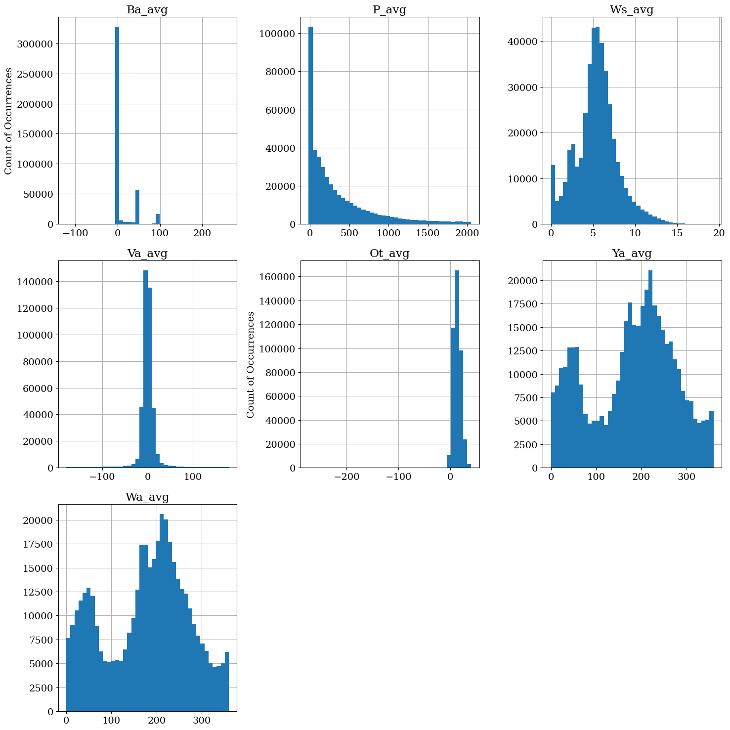
../_images/c42f16661f746f5d1ffdeb03daccd59cbefba45fc798c5bf717c0aac2f245372.png

It appears that there are a number of highly frequent values in these distributions, so we can dive into that further to see if we have some unresponsive sensors, in which case the data will need to be invalidated for later analysis. In the below analysis of repeated behaviors in the data, it seems that we should be flagging potentially unresponsive sensors (see Step 5 for more details).

# Only check data for a single turbine to avoid any spurious findings
single_turbine_df = scada_df_tz.loc[scada_df_tz.Wind_turbine_name == "R80736"].copy()

# Identify consecutive data readings
ix_consecutive = single_turbine_df.Va_avg.diff(1) != 0

# Determine how many consecutive occurences are for various thresholds, starting with 2 repeats
consecutive_counts = {i + 1: (ix_consecutive.rolling(i).sum() == 0).sum() for i in range(1, 10)}

# Plot the distribution of  N occurences for each threshold
plt.bar(consecutive_counts.keys(), consecutive_counts.values(), zorder=10)
plt.grid(zorder=0)
plt.xticks(range(2, 10))
plt.xlim((1, 10))
plt.ylim(0, 100)
plt.ylabel("Number of Consecutive Repeats")
plt.xlabel("Threshold for Consecutive Repeats")
plt.show()

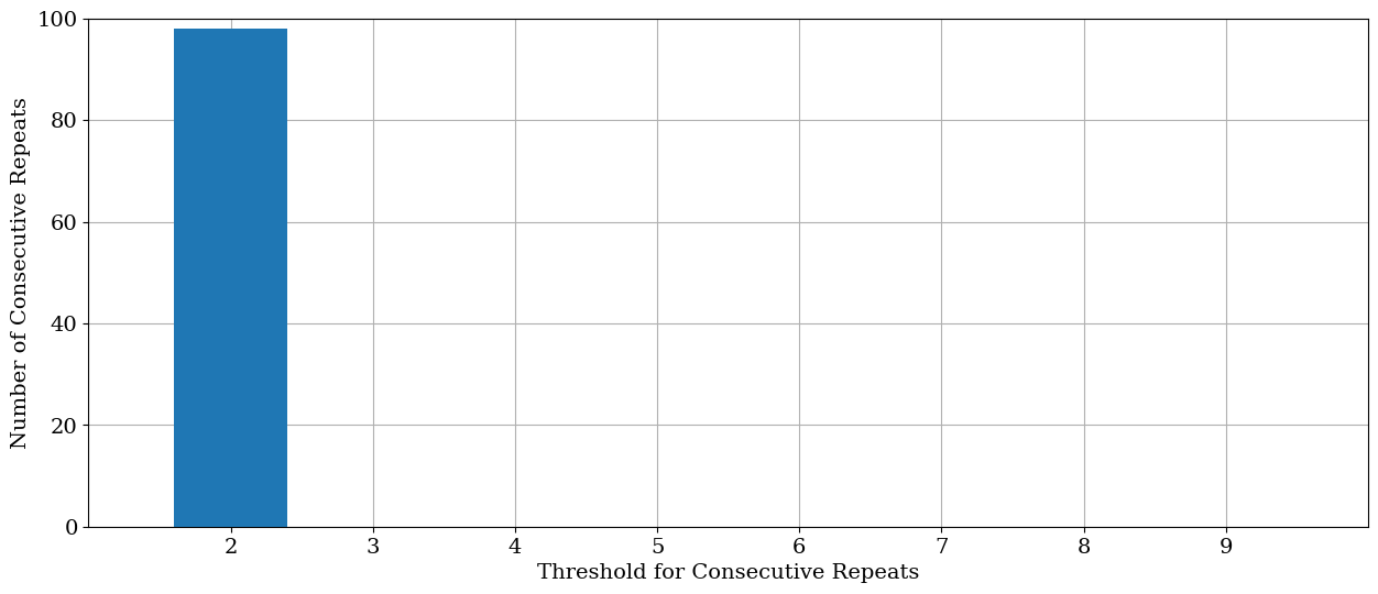
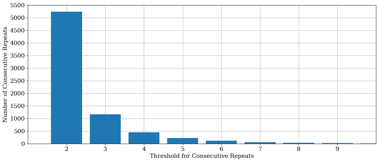
../_images/5a3ab2d86f4768b37ebb91d1e1ef7e0b9d48206e8b20d2cfca539ca9c69ec21e.png

It’s evident in the above distribution that this sensor appears to be operating adequately and won’t need to have any data flagged for unresponsiveness. However, in the below example, we can see that the temperature data are potentially having faulty data and should therefore be flagged.

# Identify consecutive data readings
ix_consecutive = single_turbine_df.Ot_avg.diff(1) != 0

# Determine how many consecutive occurences are for various thresholds, starting with 2 repeats
consecutive_counts = {i + 1: (ix_consecutive.rolling(i).sum() == 0).sum() for i in range(1, 10)}

# Plot the distribution of  N occurences for each threshold
plt.bar(consecutive_counts.keys(), consecutive_counts.values(), zorder=10)
plt.grid(zorder=0)
plt.xlim((1, 10))
plt.ylim(0, 5500)
plt.xticks(range(2, 10))
plt.yticks(range(0, 5501, 500))
plt.ylabel("Number of Consecutive Repeats")
plt.xlabel("Threshold for Consecutive Repeats")
plt.show()

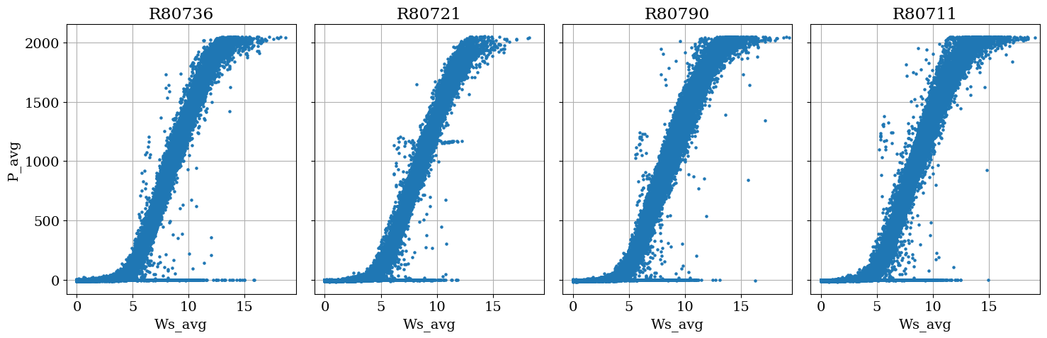
../_images/f5b5217590741d6c58c2c53d556552de52eec43204d84c063210a7f2d6b17784.png

Checking the power curve distributions#

While not contained in the QA module, the plot_by_id method is helpful for quickly assessing the quality of our operational power curves.

plot.plot_by_id(
    df=scada_df_no_tz,
    id_col="Wind_turbine_name",
    x_axis="Ws_avg",
    y_axis="P_avg",
)

../_images/41dbbe384d998386817ba5f7f6c5573bd34c924e51c712e799922c2325707eae.png

Step 4: Inspecting the timestamps for DST gaps and duplications#

Now, we can get the the duplicate time stamps from each of the data sets, according to each of the original, localized, and UTC time data. This will help us to compare the effects of DST and timezone encoding.

In the below, timezone unaware data, we can see that there is a significant deviation between the local timestamps and the UTC timestamps, especialy around the end of March in both 2018 and 2019, suggesting that there is something missing with the DST data.

Timezone-unaware data#

First we’ll look only at the data without any timezone encoding, then compare the results to the data where we kept the timezone data encoded to confirm what modifications need to be made to the data. Notice that the UTC converted data are showing duplications at roughly the same time each year when the spring-time European DST shift occurs, and is likely indicating that the original datetime stamps are missing the data to properly shift the duplicates.

dup_orig_no_tz, dup_local_no_tz, dup_utc_no_tz = qa.duplicate_time_identification(
    df=scada_df_no_tz,
    time_col="Date_time",
    id_col="Wind_turbine_name"
)
dup_orig_no_tz.size, dup_local_no_tz.size, dup_utc_no_tz.size

(48, 48, 48)

dup_utc_no_tz

Date_time_utc
2014-03-30 01:00:00+00:00   2014-03-30 01:00:00+00:00
2014-03-30 01:00:00+00:00   2014-03-30 01:00:00+00:00
2014-03-30 01:00:00+00:00   2014-03-30 01:00:00+00:00
2014-03-30 01:00:00+00:00   2014-03-30 01:00:00+00:00
2014-03-30 01:10:00+00:00   2014-03-30 01:10:00+00:00
2014-03-30 01:10:00+00:00   2014-03-30 01:10:00+00:00
2014-03-30 01:10:00+00:00   2014-03-30 01:10:00+00:00
2014-03-30 01:10:00+00:00   2014-03-30 01:10:00+00:00
2014-03-30 01:20:00+00:00   2014-03-30 01:20:00+00:00
2014-03-30 01:20:00+00:00   2014-03-30 01:20:00+00:00
2014-03-30 01:20:00+00:00   2014-03-30 01:20:00+00:00
2014-03-30 01:20:00+00:00   2014-03-30 01:20:00+00:00
2014-03-30 01:30:00+00:00   2014-03-30 01:30:00+00:00
2014-03-30 01:30:00+00:00   2014-03-30 01:30:00+00:00
2014-03-30 01:30:00+00:00   2014-03-30 01:30:00+00:00
2014-03-30 01:30:00+00:00   2014-03-30 01:30:00+00:00
2014-03-30 01:40:00+00:00   2014-03-30 01:40:00+00:00
2014-03-30 01:40:00+00:00   2014-03-30 01:40:00+00:00
2014-03-30 01:40:00+00:00   2014-03-30 01:40:00+00:00
2014-03-30 01:40:00+00:00   2014-03-30 01:40:00+00:00
2014-03-30 01:50:00+00:00   2014-03-30 01:50:00+00:00
2014-03-30 01:50:00+00:00   2014-03-30 01:50:00+00:00
2014-03-30 01:50:00+00:00   2014-03-30 01:50:00+00:00
2014-03-30 01:50:00+00:00   2014-03-30 01:50:00+00:00
2015-03-29 01:00:00+00:00   2015-03-29 01:00:00+00:00
2015-03-29 01:00:00+00:00   2015-03-29 01:00:00+00:00
2015-03-29 01:00:00+00:00   2015-03-29 01:00:00+00:00
2015-03-29 01:00:00+00:00   2015-03-29 01:00:00+00:00
2015-03-29 01:10:00+00:00   2015-03-29 01:10:00+00:00
2015-03-29 01:10:00+00:00   2015-03-29 01:10:00+00:00
2015-03-29 01:10:00+00:00   2015-03-29 01:10:00+00:00
2015-03-29 01:10:00+00:00   2015-03-29 01:10:00+00:00
2015-03-29 01:20:00+00:00   2015-03-29 01:20:00+00:00
2015-03-29 01:20:00+00:00   2015-03-29 01:20:00+00:00
2015-03-29 01:20:00+00:00   2015-03-29 01:20:00+00:00
2015-03-29 01:20:00+00:00   2015-03-29 01:20:00+00:00
2015-03-29 01:30:00+00:00   2015-03-29 01:30:00+00:00
2015-03-29 01:30:00+00:00   2015-03-29 01:30:00+00:00
2015-03-29 01:30:00+00:00   2015-03-29 01:30:00+00:00
2015-03-29 01:30:00+00:00   2015-03-29 01:30:00+00:00
2015-03-29 01:40:00+00:00   2015-03-29 01:40:00+00:00
2015-03-29 01:40:00+00:00   2015-03-29 01:40:00+00:00
2015-03-29 01:40:00+00:00   2015-03-29 01:40:00+00:00
2015-03-29 01:40:00+00:00   2015-03-29 01:40:00+00:00
2015-03-29 01:50:00+00:00   2015-03-29 01:50:00+00:00
2015-03-29 01:50:00+00:00   2015-03-29 01:50:00+00:00
2015-03-29 01:50:00+00:00   2015-03-29 01:50:00+00:00
2015-03-29 01:50:00+00:00   2015-03-29 01:50:00+00:00
Name: Date_time_utc, dtype: datetime64[ns, UTC]

To help confirm there are DST corrections needed in the data, we can also take a lot at the gaps in the timestamps, particularly in October. At a quick glance, the timezone unaware UTC encoding seems to create gaps in the data, likely accounting for the DST shift in the fall.

Based on the duplicated timestamps in the original data, it does seem like there is a DST correction in spring but no duplicate times in the fall. However, even with a UTC conversion, there still appear to be duplications in the data, so there is likely additional analysis needed here. While it appears that there are time gaps in the data for the original inputs, this phenomena switches seasons to the fall for the UTC converted time stamps, likely due to the lack of timezone encoding in the original inputs compared to a corrected timestamp.

gap_orig_no_tz, gap_local_no_tz, gap_utc_no_tz = qa.gap_time_identification(
    df=scada_df_no_tz,
    time_col="Date_time",
    freq="10min"
)
gap_orig_no_tz.size, gap_local_no_tz.size, gap_utc_no_tz.size

(12, 12, 12)

gap_orig_no_tz

  2014-03-30 02:10:00
  2014-03-30 02:20:00
  2015-03-29 02:40:00
  2015-03-29 02:30:00
  2015-03-29 02:00:00
  2014-03-30 02:40:00
  2015-03-29 02:20:00
  2014-03-30 02:00:00
  2015-03-29 02:10:00
  2014-03-30 02:30:00
 2014-03-30 02:50:00
 2015-03-29 02:50:00
Name: Date_time, dtype: datetime64[ns]

gap_utc_no_tz

  2014-10-26 01:00:00+00:00
  2015-10-25 01:00:00+00:00
  2015-10-25 01:50:00+00:00
  2015-10-25 01:10:00+00:00
  2014-10-26 01:40:00+00:00
  2015-10-25 01:30:00+00:00
  2014-10-26 01:30:00+00:00
  2015-10-25 01:40:00+00:00
  2014-10-26 01:50:00+00:00
  2014-10-26 01:20:00+00:00
 2015-10-25 01:20:00+00:00
 2014-10-26 01:10:00+00:00
Name: Date_time_utc, dtype: datetime64[ns, UTC]

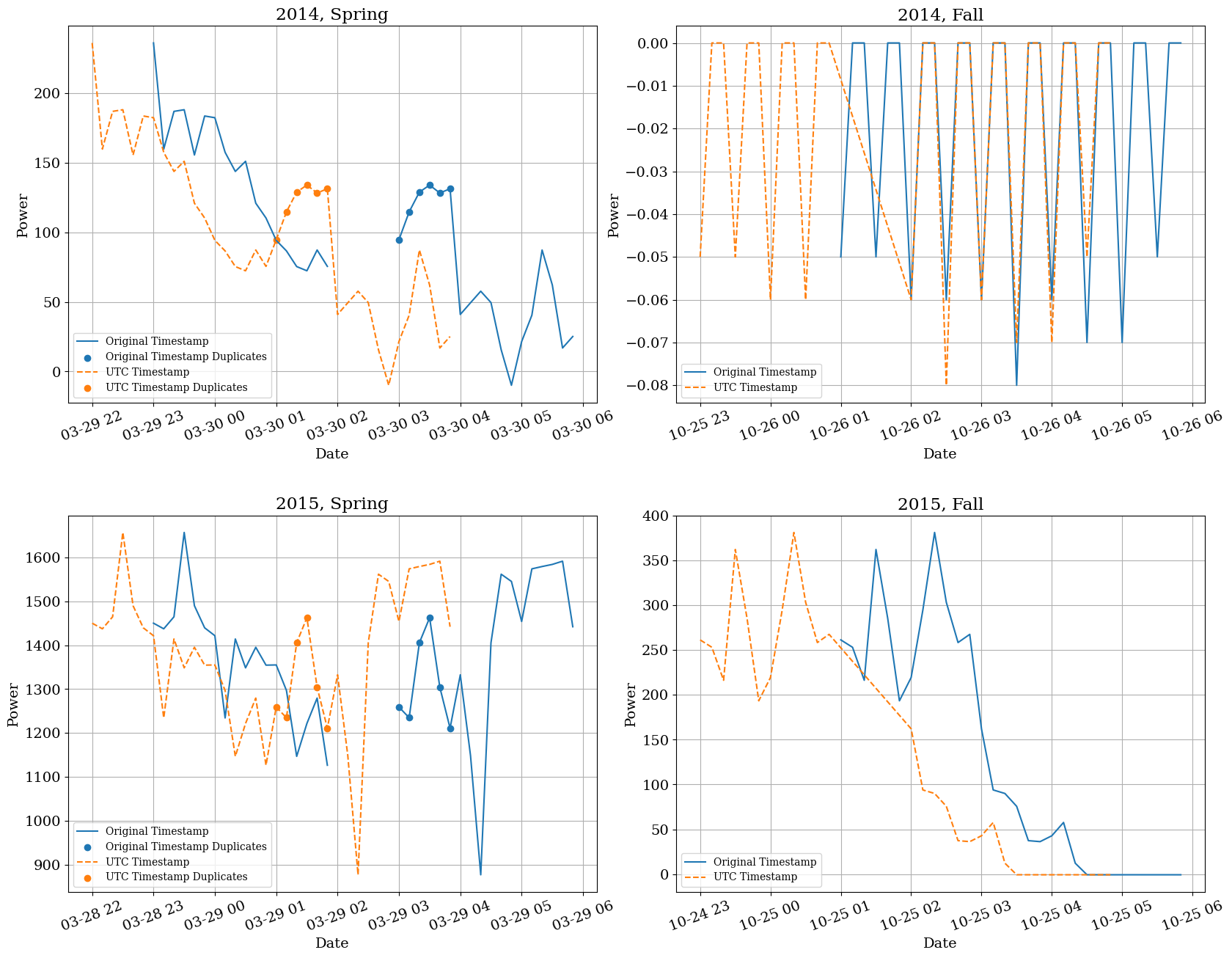
Below, we can observe the effects of not having timezones encoded, and what that might mean for potential analyses. In the unaware data, it appears that the original data (blue, solid line, labeled “Original Timestamp”) has a time gap in the spring; however, when we compare it to the UTC timestamp (orange, dashed line), it is clear that there is not in fact any gap in the data, and the DST transition has been encoded properly in the data. On the otherhand, it at first appears that there are no gaps in the fall when we make the same comparison, but when looking at the UTC timestamps, we can see that there is a 1 hour gap in the data for both 2014 and 2015. This is in line with our comparison of the original and UTC time gaps above, and further confirms our findings that there are duplicates in the spring and gaps in the fall.

By having the original data and a UTC-converted timestamp it enables us to see any gaps that may appear when there is no timezone data encoded. On the other hand, using the UTC-converted timestamp does not reduce the number of duplications in this dataset that are present in the spring, but helps adjust for seemingly missing or available data. In tandem we can see in the scatter points that there are still duplicates in the spring data just before the DST switch.

# Timezone Unaware
qa.daylight_savings_plot(
    df=scada_df_no_tz,
    local_tz="Europe/Paris",
    id_col="Wind_turbine_name",
    time_col="Date_time",
    power_col="P_avg",
    freq="10min",
    hour_window=3  # default value
)

WARNING:py.warnings:/Users/rhammond/GitHub_Public/OpenOA/openoa/utils/timeseries.py:213: FutureWarning: The behavior of DataFrame concatenation with empty or all-NA entries is deprecated. In a future version, this will no longer exclude empty or all-NA columns when determining the result dtypes. To retain the old behavior, exclude the relevant entries before the concat operation.
  data = pd.concat([data, gap_df], axis=0)

WARNING:py.warnings:/Users/rhammond/GitHub_Public/OpenOA/openoa/utils/timeseries.py:213: FutureWarning: The behavior of DataFrame concatenation with empty or all-NA entries is deprecated. In a future version, this will no longer exclude empty or all-NA columns when determining the result dtypes. To retain the old behavior, exclude the relevant entries before the concat operation.
  data = pd.concat([data, gap_df], axis=0)

../_images/1fe22662063009773b1af07bd8a88d46cbabb9e1b68ad440696fe75c241b24fc.png

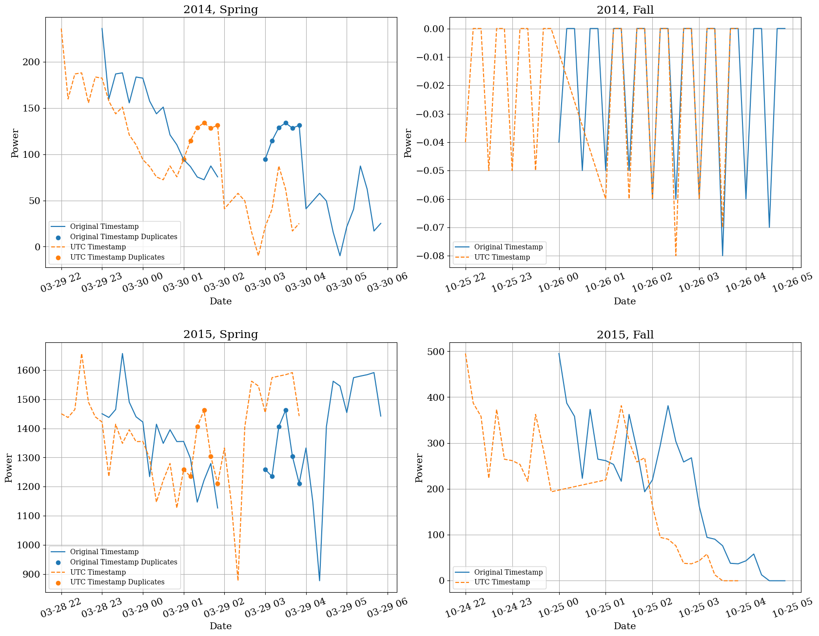
Timezone-aware data#

We see a similar finding for timezeone-aware data, below, for the both the number of duplications and gaps, likely confirming our hunches from above.

dup_orig_tz, dup_local_tz, dup_utc_tz = qa.duplicate_time_identification(
    df=scada_df_tz,
    time_col="Date_time",
    id_col="Wind_turbine_name"
)

dup_orig_tz.size, dup_local_tz.size, dup_utc_tz.size

(48, 48, 48)

dup_utc_tz

Date_time_utc
2014-03-30 01:00:00+00:00   2014-03-30 01:00:00+00:00
2014-03-30 01:00:00+00:00   2014-03-30 01:00:00+00:00
2014-03-30 01:00:00+00:00   2014-03-30 01:00:00+00:00
2014-03-30 01:00:00+00:00   2014-03-30 01:00:00+00:00
2014-03-30 01:10:00+00:00   2014-03-30 01:10:00+00:00
2014-03-30 01:10:00+00:00   2014-03-30 01:10:00+00:00
2014-03-30 01:10:00+00:00   2014-03-30 01:10:00+00:00
2014-03-30 01:10:00+00:00   2014-03-30 01:10:00+00:00
2014-03-30 01:20:00+00:00   2014-03-30 01:20:00+00:00
2014-03-30 01:20:00+00:00   2014-03-30 01:20:00+00:00
2014-03-30 01:20:00+00:00   2014-03-30 01:20:00+00:00
2014-03-30 01:20:00+00:00   2014-03-30 01:20:00+00:00
2014-03-30 01:30:00+00:00   2014-03-30 01:30:00+00:00
2014-03-30 01:30:00+00:00   2014-03-30 01:30:00+00:00
2014-03-30 01:30:00+00:00   2014-03-30 01:30:00+00:00
2014-03-30 01:30:00+00:00   2014-03-30 01:30:00+00:00
2014-03-30 01:40:00+00:00   2014-03-30 01:40:00+00:00
2014-03-30 01:40:00+00:00   2014-03-30 01:40:00+00:00
2014-03-30 01:40:00+00:00   2014-03-30 01:40:00+00:00
2014-03-30 01:40:00+00:00   2014-03-30 01:40:00+00:00
2014-03-30 01:50:00+00:00   2014-03-30 01:50:00+00:00
2014-03-30 01:50:00+00:00   2014-03-30 01:50:00+00:00
2014-03-30 01:50:00+00:00   2014-03-30 01:50:00+00:00
2014-03-30 01:50:00+00:00   2014-03-30 01:50:00+00:00
2015-03-29 01:00:00+00:00   2015-03-29 01:00:00+00:00
2015-03-29 01:00:00+00:00   2015-03-29 01:00:00+00:00
2015-03-29 01:00:00+00:00   2015-03-29 01:00:00+00:00
2015-03-29 01:00:00+00:00   2015-03-29 01:00:00+00:00
2015-03-29 01:10:00+00:00   2015-03-29 01:10:00+00:00
2015-03-29 01:10:00+00:00   2015-03-29 01:10:00+00:00
2015-03-29 01:10:00+00:00   2015-03-29 01:10:00+00:00
2015-03-29 01:10:00+00:00   2015-03-29 01:10:00+00:00
2015-03-29 01:20:00+00:00   2015-03-29 01:20:00+00:00
2015-03-29 01:20:00+00:00   2015-03-29 01:20:00+00:00
2015-03-29 01:20:00+00:00   2015-03-29 01:20:00+00:00
2015-03-29 01:20:00+00:00   2015-03-29 01:20:00+00:00
2015-03-29 01:30:00+00:00   2015-03-29 01:30:00+00:00
2015-03-29 01:30:00+00:00   2015-03-29 01:30:00+00:00
2015-03-29 01:30:00+00:00   2015-03-29 01:30:00+00:00
2015-03-29 01:30:00+00:00   2015-03-29 01:30:00+00:00
2015-03-29 01:40:00+00:00   2015-03-29 01:40:00+00:00
2015-03-29 01:40:00+00:00   2015-03-29 01:40:00+00:00
2015-03-29 01:40:00+00:00   2015-03-29 01:40:00+00:00
2015-03-29 01:40:00+00:00   2015-03-29 01:40:00+00:00
2015-03-29 01:50:00+00:00   2015-03-29 01:50:00+00:00
2015-03-29 01:50:00+00:00   2015-03-29 01:50:00+00:00
2015-03-29 01:50:00+00:00   2015-03-29 01:50:00+00:00
2015-03-29 01:50:00+00:00   2015-03-29 01:50:00+00:00
Name: Date_time_utc, dtype: datetime64[ns, UTC]

gap_orig_tz, gap_local_tz, gap_utc_tz = qa.gap_time_identification(
    df=scada_df_tz,
    time_col="Date_time",
    freq="10min"
)
gap_orig_tz.size, gap_local_tz.size, gap_utc_tz.size

(12, 12, 12)

gap_utc_tz

  2015-10-25 00:20:00+00:00
  2014-10-26 00:20:00+00:00
  2014-10-26 00:10:00+00:00
  2014-10-26 00:00:00+00:00
  2014-10-26 00:50:00+00:00
  2015-10-25 00:50:00+00:00
  2015-10-25 00:10:00+00:00
  2014-10-26 00:40:00+00:00
  2015-10-25 00:00:00+00:00
  2014-10-26 00:30:00+00:00
 2015-10-25 00:40:00+00:00
 2015-10-25 00:30:00+00:00
Name: Date_time_utc, dtype: datetime64[ns, UTC]

Again, we see a high degree of similarity between the two examples, and so can confirm that we have some duplicated data in the spring unrelated to the DST shift, and some missing data in the fall likely due to the DST shift. Additionally, we can confirm that the Europe/Paris timezone is in fact the encoding of our original data, and should therefore be converted to UTC for later analyses.

# Timezone Aware
qa.daylight_savings_plot(
    df=scada_df_tz,
    local_tz="Europe/Paris",
    id_col="Wind_turbine_name",
    time_col="Date_time",
    power_col="P_avg",
    freq="10min",
    hour_window=3  # default value
)

WARNING:py.warnings:/Users/rhammond/GitHub_Public/OpenOA/openoa/utils/timeseries.py:213: FutureWarning: The behavior of DataFrame concatenation with empty or all-NA entries is deprecated. In a future version, this will no longer exclude empty or all-NA columns when determining the result dtypes. To retain the old behavior, exclude the relevant entries before the concat operation.
  data = pd.concat([data, gap_df], axis=0)

WARNING:py.warnings:/Users/rhammond/GitHub_Public/OpenOA/openoa/utils/timeseries.py:213: FutureWarning: The behavior of DataFrame concatenation with empty or all-NA entries is deprecated. In a future version, this will no longer exclude empty or all-NA columns when determining the result dtypes. To retain the old behavior, exclude the relevant entries before the concat operation.
  data = pd.concat([data, gap_df], axis=0)

../_images/062b8df9ca039976c1263b2b9e28b83918edcbbc3261ed66ba3c1b27f933f202.png

Summarizing the QA process into a reproducible workflow#

The following description summarizes the steps taken to successfully import the ENGIE SCADA data based on the above analysis, and are implemented in the project_ENGIE.prepare() method. It should be noted that this method is cleaned up to provide users with an easy to follow example, it could also be contained in an analysis notebook, stand-alone script, etc., as long as it is able to feed into PlantData at the end of it.

From Step 2 and Step 4 we found that the data is in local time and should be converted to UTC for clarity in the timestamps. THis corresponds with line project_ENGIE.py:79.
Additionally from Step 4, it was clear that duplicated timestamp data will need to be removed, corresponding to line project_ENGIE.py:82
In Step 3, there is an oversized range for the temperature data, so this data will be invalidated, corresponding to line project_ENGIE.py:86
In Step 3, the wind vane direction (“Va_avg”) and temperature (“Ot_avg”) fields seemed to have a large number duplicated data that were identified, so these data are flagged and invalidated, which corresponds to lines project_ENGIE.py:88-102
Finally, in Step 3, it also should be noted that the pitch direction ranges from 0 to 360 degrees, and this will be corrected to the range of [-180, 180], which corresponds to lines: project_ENGIE.py:105-107

The remainder of the data do not need modification aside from additional variable calculations (see project_ENGIE.py for more details) and the aforementioned timestamp conversions.

`PlantData` demonstration#

In project_ENGIE.prepare() there are two methods to return the data: by dataframe (return_value="dataframes") and by PlantData (return_value="plantdata"), which are both demonstrated below.

For the dataframe return selection, below it is also demonstrated how to load the dataframes into a PlantData object. A couple of things to notice about the creation of the the v3 PlantData object:

metadata: This field is what maps the OpenOA column convention to the user’s column naming convention (PlantData.update_column_names(to_original=True) enables users to remap the data back to their original naming convention), in addition to a few other plant metadata objects.
analysis_type: This field controls how the data will be validated, if at all, based on the analysis requirements defined in openoa.plant.ANALYSIS_REQUIREMENTS.

scada_df, meter_df, curtail_df, asset_df, reanalysis_dict = project_ENGIE.prepare(
    path="data/la_haute_borne",
    return_value="dataframes",
    use_cleansed=False,
)

engie = PlantData(
    analysis_type=None,  # No validation desired at this point in time
    metadata="data/plant_meta.yml",
    scada=scada_df,
    meter=meter_df,
    curtail=curtail_df,
    asset=asset_df,
    reanalysis=reanalysis_dict,
)

Below is a summary of what the PlantData and PlantMetaData object specifications are, which are both new or effectively new as of version 3.0

`PlantData` documentation#

print(PlantData.__doc__)

Overarching data object used for storing, accessing, and acting on the primary
    operational analysis data types, including: SCADA, meter, tower, status, curtailment,
    asset, and reanalysis data. As of version 3.0, this class provides an automated
    validation scheme through the use of `analysis_type` as well as a secondary scheme
    that can be run after further manipulations are performed. Additionally, version 3.0
    incorporates a metadata scheme `PlantMetaData` to map between user column naming
    conventions and the internal column naming conventions for both usability and code
    consistency.

    Args:
        metadata (`PlantMetaData`): A nested dictionary of the schema definition
            for each of the data types that will be input, and some additional plant
            parameters. See ``PlantMetaData``, ``SCADAMetaData``, ``MeterMetaData``,
            ``TowerMetaData``, ``StatusMetaData``, ``CurtailMetaData``, ``AssetMetaData``,
            and/or ``ReanalysisMetaData`` for more information.
        analysis_type (`list[str]`): A single, or list of, analysis type(s) that
            will be run, that are configured in ``ANALYSIS_REQUIREMENTS``. See
            :py:attr:`openoa.schema.metadata.ANALYSIS_REQUIREMENTS` for requirements details.

            - None: Don't raise any errors for errors found in the data. This is intended
              for loading in messy data, but :py:meth:`validate` should be run later
              if planning on running any analyses.
            - "all": This is to check that all columns specified in the metadata schema
              align with the data provided, as well as data types and frequencies (where
              applicable).
            - "MonteCarloAEP": Checks the data components that are relevant to a Monte
              Carlo AEP analysis.
            - "MonteCarloAEP-temp": Checks the data components that are relevant to a
              Monte Carlo AEP analysis with ambient temperature data.
            - "MonteCarloAEP-wd": Checks the data components that are relevant to a
              Monte Carlo AEP analysis using an additional wind direction data point.
            - "MonteCarloAEP-temp-wd": Checks the data components that are relevant to a
              Monte Carlo AEP analysis with ambient temperature and wind direction data.
            - "TurbineLongTermGrossEnergy": Checks the data components that are relevant
              to a turbine long term gross energy analysis.
            - "ElectricalLosses": Checks the data components that are relevant to an
              electrical losses analysis.
            - "WakeLosses-scada": Checks the data components that are relevant to a
              wake losses analysis that uses the SCADA-based wind speed and direction
              data.
            - "WakeLosses-tower": Checks the data components that are relevant to a
              wake losses analysis that uses the met tower-based wind speed and
              direction data.

        scada (``pd.DataFrame``): Either the SCADA data that's been pre-loaded to a
            pandas `DataFrame`, or a path to the location of the data to be imported.
            See :py:class:`SCADAMetaData` for column data specifications.
        meter (``pd.DataFrame``): Either the meter data that's been pre-loaded to a
            pandas `DataFrame`, or a path to the location of the data to be imported.
            See :py:class:`MeterMetaData` for column data specifications.
        tower (``pd.DataFrame``): Either the met tower data that's been pre-loaded
            to a pandas `DataFrame`, or a path to the location of the data to be
            imported. See :py:class:`TowerMetaData` for column data specifications.
        status (``pd.DataFrame``): Either the status data that's been pre-loaded to
            a pandas `DataFrame`, or a path to the location of the data to be imported.
            See :py:class:`StatusMetaData` for column data specifications.
        curtail (``pd.DataFrame``): Either the curtailment data that's been
            pre-loaded to a pandas ``DataFrame``, or a path to the location of the data to
            be imported. See :py:class:`CurtailMetaData` for column data specifications.
        asset (``pd.DataFrame``): Either the asset summary data that's been
            pre-loaded to a pandas `DataFrame`, or a path to the location of the data to
            be imported. See :py:class:`AssetMetaData` for column data specifications.
        reanalysis (``dict[str, pd.DataFrame]``): Either the reanalysis data that's
            been pre-loaded to a dictionary of pandas ``DataFrame`` with keys indicating
            the data source, such as "era5" or "merra2", or a dictionary of paths to the
            location of the data to be imported following the same key naming convention.
            See :py:class:`ReanalysisMetaData` for column data specifications.

    Raises:
        ValueError: Raised if any analysis specific validation checks don't pass with an
            error message highlighting the appropriate issues.
    

`PlantMetaData` Documentation#

from openoa.plant import PlantMetaData
print(PlantMetaData.__doc__)

Composese the metadata/validation requirements from each of the individual data
    types that can compose a `PlantData` object.

    Args:
        latitude (`float`): The wind power plant's center point latitude.
        longitude (`float`): The wind power plant's center point longitude.
        reference_system (:obj:`str`, optional): Used to define the coordinate reference system
            (CRS). Defaults to the European Petroleum Survey Group (EPSG) code 4326 to be used with
            the World Geodetic System reference system, WGS 84.
        utm_zone (:obj:`int`, optional): UTM zone. If set to None (default), then calculated from
            the longitude.
        reference_longitude (:obj:`float`, optional): Reference longitude for calculating the UTM
            zone. If None (default), then taken as the average longitude of all assets when the
            geometry is parsed.
        capacity (`float`): The capacity of the plant in MW
        scada (`SCADAMetaData`): A dictionary containing the ``SCADAMetaData``
            column mapping and frequency parameters. See ``SCADAMetaData`` for more details.
        meter (`MeterMetaData`): A dictionary containing the ``MeterMetaData``
            column mapping and frequency parameters. See ``MeterMetaData`` for more details.
        tower (`TowerMetaData`): A dictionary containing the ``TowerMetaData``
            column mapping and frequency parameters. See ``TowerMetaData`` for more details.
        status (`StatusMetaData`): A dictionary containing the ``StatusMetaData``
            column mapping parameters. See ``StatusMetaData`` for more details.
        curtail (`CurtailMetaData`): A dictionary containing the ``CurtailMetaData``
            column mapping and frequency parameters. See ``CurtailMetaData`` for more details.
        asset (`AssetMetaData`): A dictionary containing the ``AssetMetaData``
            column mapping parameters. See ``AssetMetaData`` for more details.
        reanalysis (`dict[str, ReanalysisMetaData]`): A dictionary containing the
            reanalysis type (as keys, such as "era5" or "merra2") and ``ReanalysisMetaData``
            column mapping and frequency parameters for each type of reanalysis data
            provided. See ``ReanalysisMetaData`` for more details.
    

`PlantData` validation#

Because PlantData is an attrs dataclass, it enables to support automatic conversion and validation of variables, which enables users to change analysis types as they work through their data. Below is a demonstration of what happens when we add an invalid analysis type (which fails to enable it), add the “MonteCarloAEP” analysis type (which passes the validation), and then further add in the “all” analysis type (which fails).

try:
    engie.analysis_type = "MonteCarlo"
except ValueError as e:
    print(e)

("'analysis_type' must be in ['MonteCarloAEP', 'MonteCarloAEP-temp', 'MonteCarloAEP-wd', 'MonteCarloAEP-temp-wd', 'TurbineLongTermGrossEnergy', 'ElectricalLosses', 'WakeLosses-scada', 'WakeLosses-tower', 'StaticYawMisalignment', 'all', None] (got 'MonteCarlo')", Attribute(name='analysis_type', default=None, validator=<deep_iterable validator for <instance_of validator for type <class 'list'>> iterables of <in_ validator with options ['MonteCarloAEP', 'MonteCarloAEP-temp', 'MonteCarloAEP-wd', 'MonteCarloAEP-temp-wd', 'TurbineLongTermGrossEnergy', 'ElectricalLosses', 'WakeLosses-scada', 'WakeLosses-tower', 'StaticYawMisalignment', 'all', None]>>, repr=True, eq=True, eq_key=None, order=True, order_key=None, hash=None, init=True, metadata=mappingproxy({}), type='list[str] | None', converter=<function convert_to_list at 0x127ffaac0>, kw_only=False, inherited=False, on_setattr=<function pipe.<locals>.wrapped_pipe at 0x127ffb4c0>, alias='analysis_type'), ['MonteCarloAEP', 'MonteCarloAEP-temp', 'MonteCarloAEP-wd', 'MonteCarloAEP-temp-wd', 'TurbineLongTermGrossEnergy', 'ElectricalLosses', 'WakeLosses-scada', 'WakeLosses-tower', 'StaticYawMisalignment', 'all', None], 'MonteCarlo')

engie.analysis_type = "MonteCarloAEP"
engie.validate()

Notice that in the above cell, the data validates successfully for the MonteCarloAEP analysis, but below, when we append the "all" type, the validation fails. The below failure is because when "all" is input to analysis_type, it checks all of the data, and not just the analysis categories. In this case, there are no inputs to tower and status, so each of the checks will fail for all of the required columns by the metadata classifications.

engie.analysis_type.append("all")
print(f"The new analysis types now has all and MonteCarloAEP: {engie.analysis_type}")
try:
    engie.validate()
except ValueError as e: # Catch the error message so that the whole notebook can run
    print(e)

The new analysis types now has all and MonteCarloAEP: ['MonteCarloAEP', 'all']
`scada` data is missing the following columns: ['WTUR_TurSt']
`tower` data is missing the following columns: ['time', 'asset_id', 'WMET_HorWdSpd', 'WMET_HorWdDir', 'WMET_EnvTmp']
`status` data is missing the following columns: ['time', 'asset_id', 'status_id', 'status_code', 'status_text']
`scada` data columns were of the wrong type: ['WTUR_TurSt']
`tower` data columns were of the wrong type: ['time', 'asset_id', 'WMET_HorWdSpd', 'WMET_HorWdDir', 'WMET_EnvTmp']
`status` data columns were of the wrong type: ['time', 'asset_id', 'status_id', 'status_code', 'status_text']

Below, the ENGIE data has been re-validated for a “MonteCarloAEP” analysis, so that it can be saved for later, and reloaded as the cleaned up version for easier importing.

engie.analysis_type = "MonteCarloAEP"
engie.validate()

data_path = "data/cleansed"
engie.to_csv(save_path=data_path, with_openoa_col_names=True)

engie_clean = PlantData(
    metadata=f"{data_path}/metadata.yml",
    scada=f"{data_path}/scada.csv",
    meter=f"{data_path}/meter.csv",
    curtail=f"{data_path}/curtail.csv",
    asset=f"{data_path}/asset.csv",
    reanalysis={
        "era5": f"{data_path}/reanalysis_era5.csv",
        "merra2": f"{data_path}/reanalysis_merra2.csv"
    },
)

`PlantData` string and markdown representations#

Below, we can see a summary of all the data contained in the PlantData object, engie_clean.

print(engie_clean)

analysis_type: [None]

scada
-----
+------------------+-------------+---------+---------+----------+---------+---------+---------+-----------+
|                  |       count |    mean |     std |      min |     25% |     50% |     75% |       max |
+==================+=============+=========+=========+==========+=========+=========+=========+===========+
| WROT_BlPthAngVal | 417,820.000 |  10.032 |  23.231 | -165.310 |  -0.990 |  -0.990 |   0.140 |   120.040 |
+------------------+-------------+---------+---------+----------+---------+---------+---------+-----------+
| WTUR_W           | 417,820.000 | 353.617 | 430.369 |  -17.920 |  35.370 | 192.160 | 508.310 | 2,051.870 |
+------------------+-------------+---------+---------+----------+---------+---------+---------+-----------+
| WMET_HorWdSpd    | 417,820.000 |   5.447 |   2.487 |    0.000 |   4.100 |   5.450 |   6.770 |    19.310 |
+------------------+-------------+---------+---------+----------+---------+---------+---------+-----------+
| WMET_HorWdDirRel | 417,820.000 |   0.114 |  23.033 | -179.950 |  -5.880 |  -0.200 |   5.900 |   179.990 |
+------------------+-------------+---------+---------+----------+---------+---------+---------+-----------+
| WMET_EnvTmp      | 417,708.000 |  12.733 |   7.168 |   -6.260 |   7.300 |  12.510 |  17.470 |    39.890 |
+------------------+-------------+---------+---------+----------+---------+---------+---------+-----------+
| Ya_avg           | 417,820.000 | 179.905 |  93.165 |    0.000 | 105.190 | 194.340 | 247.400 |   360.000 |
+------------------+-------------+---------+---------+----------+---------+---------+---------+-----------+
| WMET_HorWdDir    | 417,820.000 | 177.995 |  92.455 |    0.000 | 103.640 | 191.470 | 243.740 |   360.000 |
+------------------+-------------+---------+---------+----------+---------+---------+---------+-----------+
| energy_kwh       | 417,820.000 |  58.936 |  71.728 |   -2.987 |   5.895 |  32.027 |  84.718 |   341.978 |
+------------------+-------------+---------+---------+----------+---------+---------+---------+-----------+
| WTUR_SupWh       | 417,820.000 |  58.936 |  71.728 |   -2.987 |   5.895 |  32.027 |  84.718 |   341.978 |
+------------------+-------------+---------+---------+----------+---------+---------+---------+-----------+

meter
-----
+------------+-------------+---------+---------+--------+--------+---------+---------+-----------+
|            |       count |    mean |     std |    min |    25% |     50% |     75% |       max |
+============+=============+=========+=========+========+========+=========+=========+===========+
| MMTR_SupWh | 105,120.000 | 229.579 | 271.906 | -8.893 | 27.764 | 130.635 | 331.149 | 1,347.182 |
+------------+-------------+---------+---------+--------+--------+---------+---------+-----------+

tower
-----
no data

status
------
no data

curtail
-------
+-----------------+-------------+---------+---------+--------+--------+---------+---------+-----------+
|                 |       count |    mean |     std |    min |    25% |     50% |     75% |       max |
+=================+=============+=========+=========+========+========+=========+=========+===========+
| net_energy_kwh  | 105,120.000 | 229.579 | 271.906 | -8.893 | 27.764 | 130.635 | 331.149 | 1,347.182 |
+-----------------+-------------+---------+---------+--------+--------+---------+---------+-----------+
| IAVL_DnWh       | 105,120.000 |   2.928 |  21.549 |  0.000 |  0.000 |   0.000 |   0.000 |   828.190 |
+-----------------+-------------+---------+---------+--------+--------+---------+---------+-----------+
| IAVL_ExtPwrDnWh | 105,120.000 |   0.162 |   9.805 |  0.000 |  0.000 |   0.000 |   0.000 | 1,012.886 |
+-----------------+-------------+---------+---------+--------+--------+---------+---------+-----------+

asset
-----
+--------+------------+-------------+-------------+---------------+--------------+------------------+----------------+---------+---------+
|        |   latitude |   longitude |   elevation |   rated_power |   hub_height |   rotor_diameter | Manufacturer   | Model   | type    |
+========+============+=============+=============+===============+==============+==================+================+=========+=========+
| R80711 |     48.457 |       5.585 |     411.000 |     2,050.000 |       80.000 |           82.000 | Senvion        | MM82    | turbine |
+--------+------------+-------------+-------------+---------------+--------------+------------------+----------------+---------+---------+
| R80721 |     48.450 |       5.587 |     411.000 |     2,050.000 |       80.000 |           82.000 | Senvion        | MM82    | turbine |
+--------+------------+-------------+-------------+---------------+--------------+------------------+----------------+---------+---------+
| R80736 |     48.446 |       5.593 |     411.000 |     2,050.000 |       80.000 |           82.000 | Senvion        | MM82    | turbine |
+--------+------------+-------------+-------------+---------------+--------------+------------------+----------------+---------+---------+
| R80790 |     48.454 |       5.588 |     411.000 |     2,050.000 |       80.000 |           82.000 | Senvion        | MM82    | turbine |
+--------+------------+-------------+-------------+---------------+--------------+------------------+----------------+---------+---------+

reanalysis
----------

era5
+-----------------+-------------+------------+---------+------------+------------+------------+------------+-------------+
|                 |       count |       mean |     std |        min |        25% |        50% |        75% |         max |
+=================+=============+============+=========+============+============+============+============+=============+
| WMETR_HorWdSpdU | 187,172.000 |      1.139 |   4.729 |    -14.982 |     -2.369 |      1.436 |      4.618 |      26.079 |
+-----------------+-------------+------------+---------+------------+------------+------------+------------+-------------+
| WMETR_HorWdSpdV | 187,172.000 |      1.108 |   4.399 |    -12.953 |     -2.338 |      0.765 |      4.351 |      20.692 |
+-----------------+-------------+------------+---------+------------+------------+------------+------------+-------------+
| WMETR_EnvTmp    | 187,172.000 |    283.566 |   7.539 |    258.218 |    277.955 |    283.392 |    288.874 |     312.173 |
+-----------------+-------------+------------+---------+------------+------------+------------+------------+-------------+
| WMETR_EnvPres   | 187,172.000 | 97,740.654 | 817.576 | 93,459.055 | 97,284.750 | 97,790.907 | 98,266.866 | 100,383.261 |
+-----------------+-------------+------------+---------+------------+------------+------------+------------+-------------+
| ws_100m         | 187,172.000 |      6.041 |   2.784 |      0.003 |      4.048 |      5.810 |      7.731 |      26.795 |
+-----------------+-------------+------------+---------+------------+------------+------------+------------+-------------+
| dens_100m       | 187,172.000 |      1.198 |   0.035 |      1.071 |      1.173 |      1.196 |      1.223 |       1.331 |
+-----------------+-------------+------------+---------+------------+------------+------------+------------+-------------+
| WMETR_HorWdDir  | 187,172.000 |    185.846 |  95.604 |      0.002 |     89.797 |    206.692 |    255.341 |     359.993 |
+-----------------+-------------+------------+---------+------------+------------+------------+------------+-------------+
| WMETR_HorWdSpd  | 187,172.000 |      6.041 |   2.784 |      0.003 |      4.048 |      5.810 |      7.731 |      26.795 |
+-----------------+-------------+------------+---------+------------+------------+------------+------------+-------------+
| WMETR_AirDen    | 187,172.000 |      1.198 |   0.035 |      1.071 |      1.173 |      1.196 |      1.223 |       1.331 |
+-----------------+-------------+------------+---------+------------+------------+------------+------------+-------------+

merra2
+--------------------------+-------------+------------+---------+------------+------------+------------+------------+-------------+
|                          |       count |       mean |     std |        min |        25% |        50% |        75% |         max |
+==========================+=============+============+=========+============+============+============+============+=============+
| WMETR_EnvPres            | 195,720.000 | 97,824.122 | 826.941 | 93,182.590 | 97,355.545 | 97,875.530 | 98,361.080 | 100,470.664 |
+--------------------------+-------------+------------+---------+------------+------------+------------+------------+-------------+
| surface_skin_temperature | 195,720.000 |    282.452 |   8.331 |    254.834 |    276.159 |    281.946 |    288.411 |     317.590 |
+--------------------------+-------------+------------+---------+------------+------------+------------+------------+-------------+
| u_10                     | 195,720.000 |      1.097 |   3.338 |    -11.577 |     -1.379 |      1.082 |      3.255 |      22.332 |
+--------------------------+-------------+------------+---------+------------+------------+------------+------------+-------------+
| v_10                     | 195,720.000 |      0.805 |   3.231 |    -11.732 |     -1.628 |      0.665 |      2.996 |      17.006 |
+--------------------------+-------------+------------+---------+------------+------------+------------+------------+-------------+
| WMETR_HorWdSpdU          | 195,720.000 |      1.472 |   4.741 |    -15.337 |     -2.049 |      1.605 |      4.862 |      28.249 |
+--------------------------+-------------+------------+---------+------------+------------+------------+------------+-------------+
| WMETR_HorWdSpdV          | 195,720.000 |      1.135 |   4.570 |    -15.306 |     -2.412 |      0.962 |      4.533 |      21.851 |
+--------------------------+-------------+------------+---------+------------+------------+------------+------------+-------------+
| WMETR_EnvTmp             | 195,720.000 |    282.515 |   7.856 |    255.915 |    276.469 |    282.276 |    288.369 |     311.673 |
+--------------------------+-------------+------------+---------+------------+------------+------------+------------+-------------+
| temp_10m                 | 195,720.000 |    282.771 |   7.738 |    256.412 |    276.764 |    282.620 |    288.595 |     310.308 |
+--------------------------+-------------+------------+---------+------------+------------+------------+------------+-------------+
| u_850                    | 195,720.000 |      3.986 |   7.921 |    -30.371 |     -1.100 |      3.671 |      8.856 |      41.947 |
+--------------------------+-------------+------------+---------+------------+------------+------------+------------+-------------+
| v_850                    | 195,720.000 |      0.668 |   5.898 |    -25.058 |     -3.141 |      0.383 |      4.078 |      34.965 |
+--------------------------+-------------+------------+---------+------------+------------+------------+------------+-------------+
| temp_850                 | 195,720.000 |    277.566 |   6.395 |    254.825 |    272.997 |    277.754 |    282.130 |     298.494 |
+--------------------------+-------------+------------+---------+------------+------------+------------+------------+-------------+
| ws_50m                   | 195,720.000 |      6.170 |   2.958 |      0.027 |      4.067 |      5.951 |      7.861 |      29.404 |
+--------------------------+-------------+------------+---------+------------+------------+------------+------------+-------------+
| dens_50m                 | 195,720.000 |      1.204 |   0.037 |      1.082 |      1.177 |      1.202 |      1.230 |       1.351 |
+--------------------------+-------------+------------+---------+------------+------------+------------+------------+-------------+
| WMETR_HorWdDir           | 195,720.000 |    187.820 |  95.804 |      0.001 |     99.541 |    209.234 |    256.224 |     359.999 |
+--------------------------+-------------+------------+---------+------------+------------+------------+------------+-------------+
| WMETR_HorWdSpd           | 195,720.000 |      6.170 |   2.958 |      0.027 |      4.067 |      5.951 |      7.861 |      29.404 |
+--------------------------+-------------+------------+---------+------------+------------+------------+------------+-------------+
| WMETR_AirDen             | 195,720.000 |      1.204 |   0.037 |      1.082 |      1.177 |      1.202 |      1.230 |       1.351 |
+--------------------------+-------------+------------+---------+------------+------------+------------+------------+-------------+

While this is really great, it is a bit more catered towards a terminal output, and so we provide a Jupyter-friendly Markdown representation as well, as can be seen below. Alternatively, engie_clean.markdown() can be called to ensure the data are correctly displayed in their markdown format.

NOTE: the output displayed here that is viewable on the documentation site does not display the markdown correctly, so please take a look at the actual notebook on the GitHub or in your own Jupyter session.

engie_clean

PlantData

analysis_type

None

asset

| asset_id | latitude | longitude | elevation | rated_power | hub_height | rotor_diameter | Manufacturer | Model | type | |:———–|———–:|————:|————:|————–:|————-:|—————–:|:—————|:——–|:——–| | R80711 | 48.4569 | 5.5847 | 411 | 2050 | 80 | 82 | Senvion | MM82 | turbine | | R80721 | 48.4497 | 5.5869 | 411 | 2050 | 80 | 82 | Senvion | MM82 | turbine | | R80736 | 48.4461 | 5.5925 | 411 | 2050 | 80 | 82 | Senvion | MM82 | turbine | | R80790 | 48.4536 | 5.5875 | 411 | 2050 | 80 | 82 | Senvion | MM82 | turbine |

scada

| | count | mean | std | min | 25% | 50% | 75% | max | |:—————–|——–:|———-:|———-:|———–:|——–:|———:|———:|———:| | WROT_BlPthAngVal | 417820 | 10.0316 | 23.2314 | -165.31 | -0.99 | -0.99 | 0.14 | 120.04 | | WTUR_W | 417820 | 353.617 | 430.369 | -17.92 | 35.37 | 192.16 | 508.31 | 2051.87 | | WMET_HorWdSpd | 417820 | 5.44747 | 2.4873 | 0 | 4.1 | 5.45 | 6.77 | 19.31 | | WMET_HorWdDirRel | 417820 | 0.1138 | 23.0329 | -179.95 | -5.88 | -0.2 | 5.9 | 179.99 | | WMET_EnvTmp | 417708 | 12.7333 | 7.16816 | -6.26 | 7.3 | 12.51 | 17.47 | 39.89 | | Ya_avg | 417820 | 179.905 | 93.1649 | 0 | 105.19 | 194.34 | 247.4 | 360 | | WMET_HorWdDir | 417820 | 177.995 | 92.4553 | 0 | 103.64 | 191.47 | 243.74 | 360 | | energy_kwh | 417820 | 58.9361 | 71.7281 | -2.98667 | 5.895 | 32.0267 | 84.7183 | 341.978 | | WTUR_SupWh | 417820 | 58.9361 | 71.7281 | -2.98667 | 5.895 | 32.0267 | 84.7183 | 341.978 |

meter

| | count | mean | std | min | 25% | 50% | 75% | max | |:———–|——–:|——–:|——–:|——-:|——–:|——–:|——–:|——–:| | MMTR_SupWh | 105120 | 229.579 | 271.906 | -8.893 | 27.7635 | 130.635 | 331.149 | 1347.18 |

tower

no data

status

no data

curtail

| | count | mean | std | min | 25% | 50% | 75% | max | |:—————-|——–:|———–:|———-:|——-:|——–:|——–:|——–:|——–:| | net_energy_kwh | 105120 | 229.579 | 271.906 | -8.893 | 27.7635 | 130.635 | 331.149 | 1347.18 | | IAVL_DnWh | 105120 | 2.92777 | 21.5486 | 0 | 0 | 0 | 0 | 828.19 | | IAVL_ExtPwrDnWh | 105120 | 0.161518 | 9.80474 | 0 | 0 | 0 | 0 | 1012.89 |

reanalysis

era5

| | count | mean | std | min | 25% | 50% | 75% | max | |:—————-|——–:|————:|————:|—————:|————:|————-:|————:|————-:| | WMETR_HorWdSpdU | 187172 | 1.13927 | 4.72926 | -14.9816 | -2.36933 | 1.43596 | 4.61772 | 26.0787 | | WMETR_HorWdSpdV | 187172 | 1.10765 | 4.39909 | -12.9526 | -2.33807 | 0.765297 | 4.35094 | 20.6916 | | WMETR_EnvTmp | 187172 | 283.566 | 7.53883 | 258.218 | 277.955 | 283.392 | 288.874 | 312.173 | | WMETR_EnvPres | 187172 | 97740.7 | 817.576 | 93459.1 | 97284.7 | 97790.9 | 98266.9 | 100383 | | ws_100m | 187172 | 6.04099 | 2.7837 | 0.00328114 | 4.04821 | 5.80999 | 7.73064 | 26.7948 | | dens_100m | 187172 | 1.19845 | 0.0352755 | 1.0707 | 1.17348 | 1.19645 | 1.22293 | 1.33056 | | WMETR_HorWdDir | 187172 | 185.846 | 95.604 | 0.00191019 | 89.7974 | 206.692 | 255.341 | 359.993 | | WMETR_HorWdSpd | 187172 | 6.04099 | 2.7837 | 0.00328114 | 4.04821 | 5.80999 | 7.73064 | 26.7948 | | WMETR_AirDen | 187172 | 1.19842 | 0.0352745 | 1.07067 | 1.17344 | 1.19641 | 1.2229 | 1.33053 |

merra2

| | count | mean | std | min | 25% | 50% | 75% | max | |:————————-|——–:|————-:|————:|—————-:|————:|————-:|————:|————-:| | WMETR_EnvPres | 195720 | 97824.1 | 826.941 | 93182.6 | 97355.5 | 97875.5 | 98361.1 | 100471 | | surface_skin_temperature | 195720 | 282.452 | 8.33084 | 254.834 | 276.159 | 281.946 | 288.411 | 317.59 | | u_10 | 195720 | 1.0973 | 3.33816 | -11.577 | -1.37919 | 1.08179 | 3.25537 | 22.3319 | | v_10 | 195720 | 0.805023 | 3.23138 | -11.7316 | -1.62791 | 0.664757 | 2.99603 | 17.0065 | | WMETR_HorWdSpdU | 195720 | 1.47187 | 4.7413 | -15.3375 | -2.04887 | 1.60502 | 4.86207 | 28.2489 | | WMETR_HorWdSpdV | 195720 | 1.13452 | 4.57016 | -15.3061 | -2.41186 | 0.961586 | 4.53251 | 21.8515 | | WMETR_EnvTmp | 195720 | 282.515 | 7.85631 | 255.915 | 276.469 | 282.276 | 288.369 | 311.673 | | temp_10m | 195720 | 282.771 | 7.73835 | 256.412 | 276.764 | 282.62 | 288.595 | 310.308 | | u_850 | 195720 | 3.98599 | 7.92127 | -30.3709 | -1.09976 | 3.67055 | 8.85558 | 41.9465 | | v_850 | 195720 | 0.667629 | 5.89822 | -25.0578 | -3.14127 | 0.382695 | 4.07756 | 34.9646 | | temp_850 | 195720 | 277.566 | 6.39469 | 254.825 | 272.997 | 277.754 | 282.13 | 298.494 | | ws_50m | 195720 | 6.16986 | 2.95847 | 0.0271478 | 4.06728 | 5.95081 | 7.86064 | 29.4037 | | dens_50m | 195720 | 1.2042 | 0.0369871 | 1.08193 | 1.17673 | 1.20233 | 1.23045 | 1.35085 | | WMETR_HorWdDir | 195720 | 187.82 | 95.8037 | 0.000978537 | 99.5413 | 209.234 | 256.224 | 359.999 | | WMETR_HorWdSpd | 195720 | 6.16986 | 2.95847 | 0.0271478 | 4.06728 | 5.95081 | 7.86064 | 29.4037 | | WMETR_AirDen | 195720 | 1.20417 | 0.036986 | 1.0819 | 1.1767 | 1.20229 | 1.23041 | 1.35082 |

None

Intro to the OpenOA PlantData and QA Methods#

The PlantData object#